Motion Heatmaps from Time-Lapse Photography - Blog

January 5, 2016 / 9:46 PM

Motion Heatmaps from Time-Lapse Photography

projects

Given a sequence of N frames, each of constant dimensions, how can the amount of motion at each region of the image across the entire sequence be quantified and visualized in an intuitive way?

This is the core problem statement that this algorithm attempts to solve. Here, I present a method of visualizing the amount of motion across frames of a time-lapse photography sequence with a red-blue motion "heatmap."

A Python implementation is available on GitHub, so you can try it on your own time-lapse sequences.

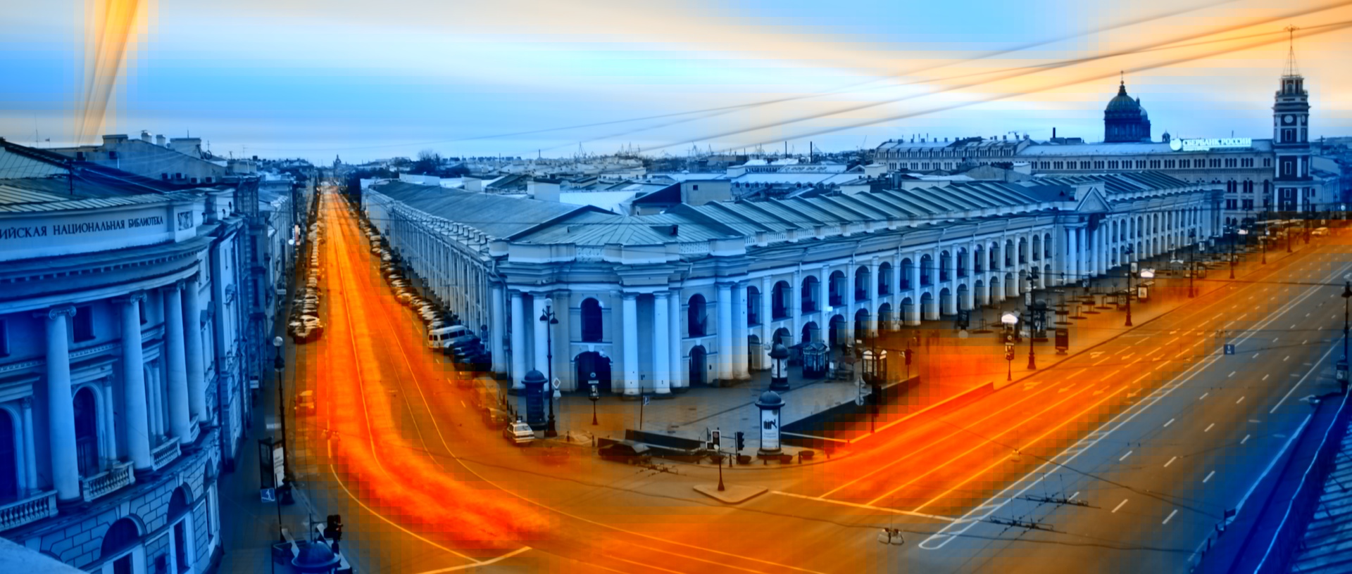
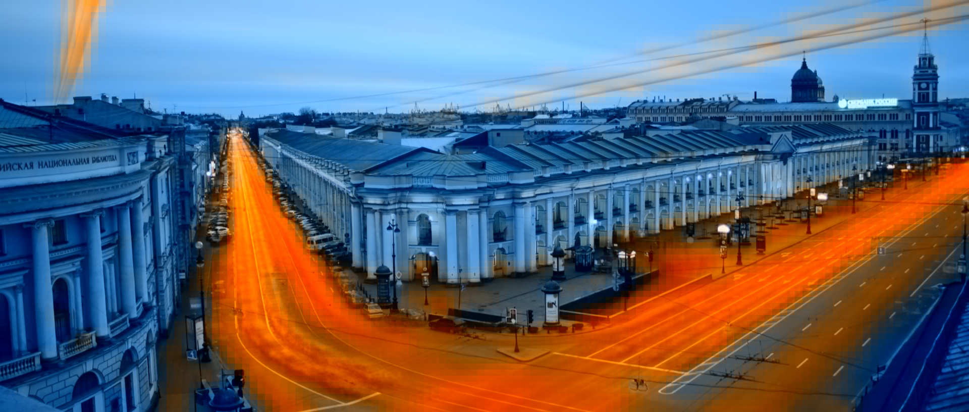
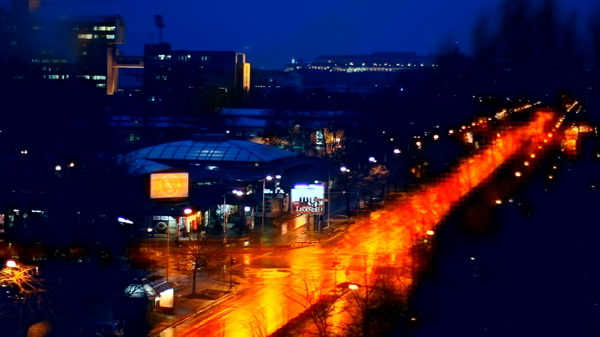
See the following for some examples of time-lapse sequences and the motion heatmaps generated using this algorithm:

The algorithm involves the following procedures, each of which is explained with more technical detail below:

Divide the frame into equal-sized blocks to represent the motion in that area of the frame

For each block, select a random pixel, and generate a signal of the grayscale intensity of at that pixel as a function of time (e.g. as a function of the frame number)

Applying a high-pass filter to each signal to reduce the impact of low-frequency motion

Calculate the standard deviation of each signal to quantify the amount of motion per block

Low-pass filter the resulting two-dimensional heatmap in order to create a more visually consistent result

Generate an overlay image by using the values of the heatmap to offset the values of the red and blue channels in each pixel of the input image

Segmenting the input into motion regions

Motion in an image is best described in terms of the general regions of the frame in which motion exists. This algorithm takes the approach of segmenting the frame into equal-sized rectangular blocks, and considering a randomly selected pixel within each of these regions to be representative of that block. The extent of motion calculated from that single pixel across all frames in the sequence is the approximate estimate of motion within that rectangular region.

The limit of this approach (e.g. a maximally precise segmentation of the input image) is the case when the rectangular region is exactly one pixel in size. While this is computationally achievable, such a segmentation no longer conveys the concept of having "regions" of motion, since each pixel from the input image is in itself the motion region.

Extracting motion data from frames

On a high level, the input is a three-dimensional matrix of dimensions w x h x N, where each index (i, j, k) represents the grayscale intensity of the image at the pixel (i, j) of frame k. The output is a two-dimensional matrix of dimensions w x h, with each pixel (i, j) color-adjusted by applying appropriate offsets to the red and blue channels that represent the extent of motion at (i, j).

Given the segmentation above, we can generate num_horizontal_divisions * num_vertical_divisions signals representing the grayscale intensity at a particular pixel as a function of the frame number (a discrete-time axis). Signals with mostly low-frequency content can be considered to have little or no motion, whereas signals with significant high-frequency content can be considered to have more motion.

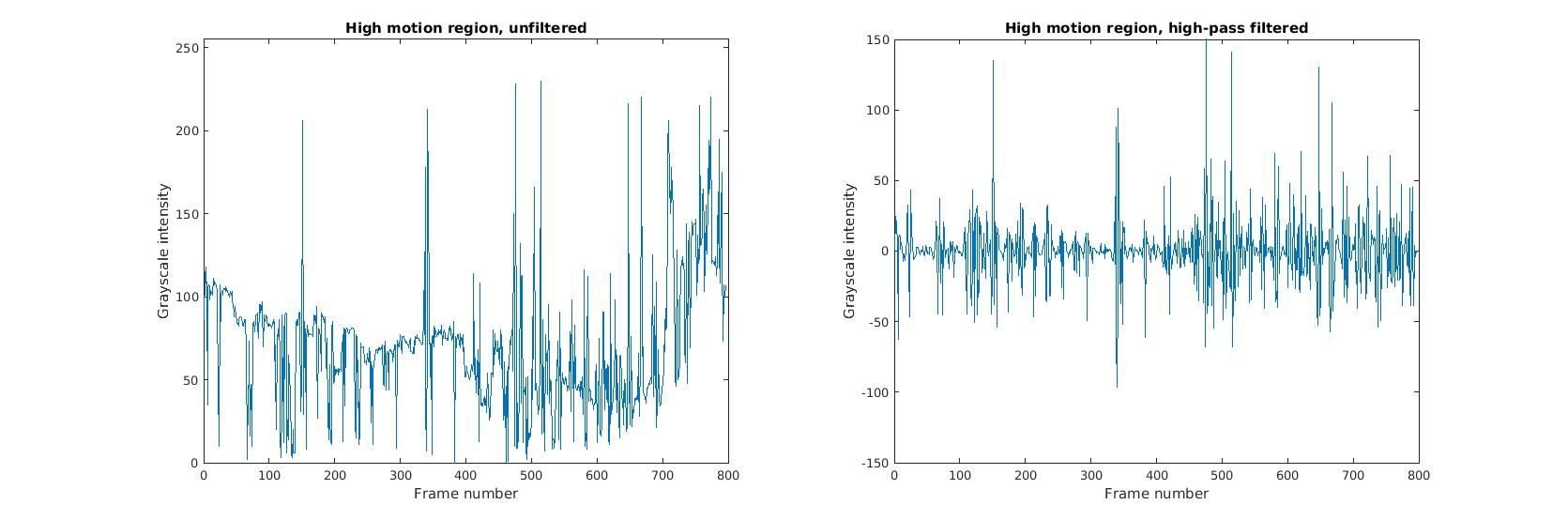
This approach works well for accurately measuring the variance in a region across the entire sequence. However, a practical consideration for time-lapse photography is handling the effects of small, incremental changes in the scene across a long period of time: for example, the lighting may slowly change from daytime to nighttime, or there may be small changes in the position of the frame due to camera shake. These small perturbations contribute to the pixel variance, albeit to a lesser extent than actual motion. A straightforward way to counteract these small, low-frequency events is to apply as high-pass filter to each of the signals before calculating its variance. This reduces the impact of incremental changes on the heatmap, while still preserving the core information on actual motion that occurs across frames.

This algorithm applies a Butterworth filter of the noted parameters to each of the signals:

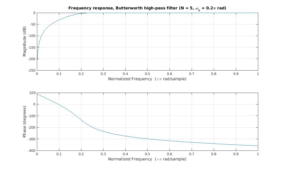
The filter eliminates the effects of small slopes in the grayscale intensity (e.g. from gradual daylight transitions) and eliminates DC offsets while preserving data on significant, high-frequency changes.

Quantifying per-pixel variance and generating a heatmap

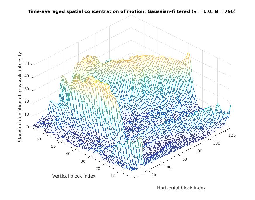
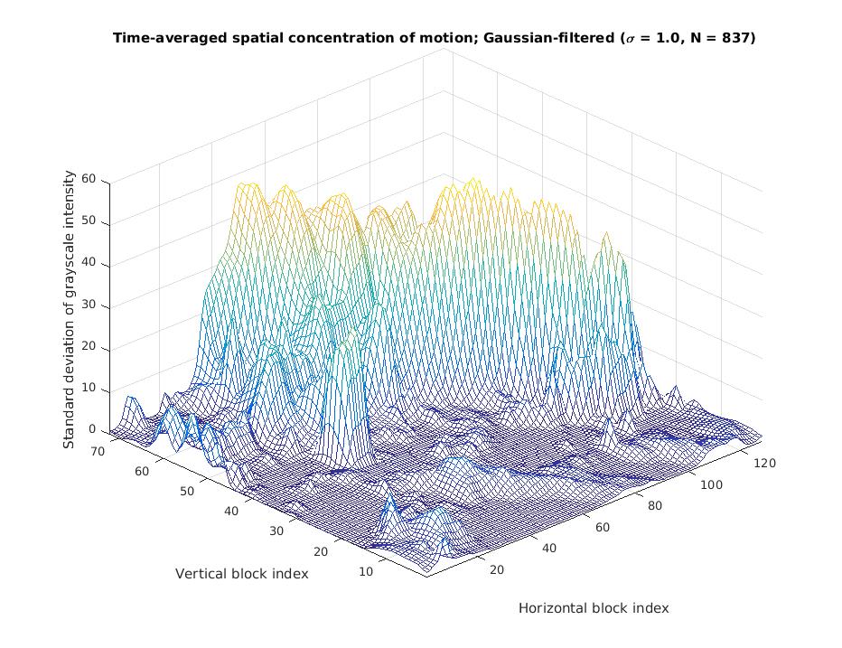
This algorithm considers only the standard deviation of each of the signals as described above across all frames as a quantitative measure of the amount of motion at any particular pixel. (A more interesting approach might take the FFT of each of these signals for frequency-domain analysis; the amount of power within different "bins" of frequency might correspond to the amount of RGB offset on each motion region.)

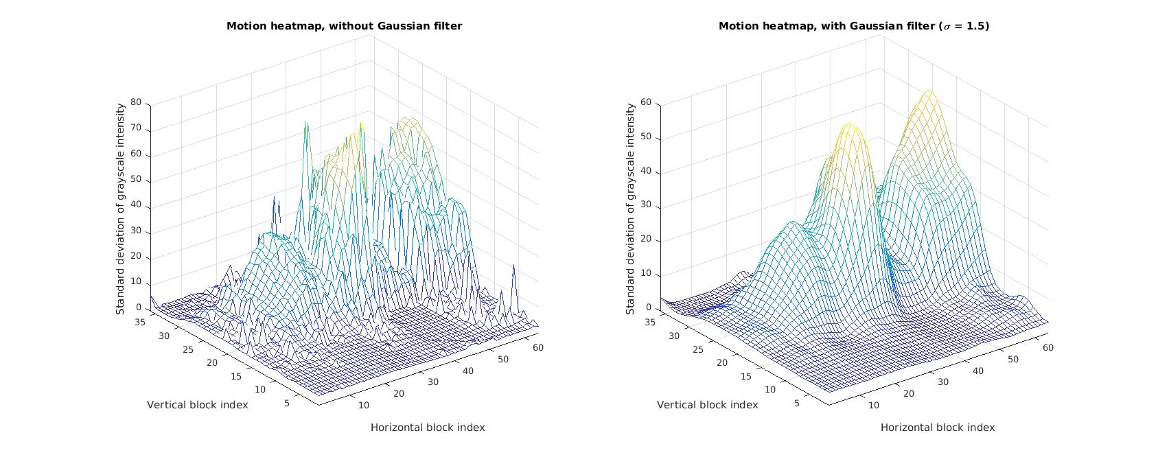
From this data, we can generate a three-dimensional heatmap indicating the standard deviation at each of the motion regions (a spatial plane). The values on this heatmap at each motion region correlate directly to the amount of red and blue offset in the final heatmap overlay image. However, in order to reduce the visual inconsistency caused by regions with a high standard deviation relative to its neighbors (e.g. high-frequency content), we apply a low-pass Gaussian filter to the heatmap before using it as input to generating the heatmap overlay image.

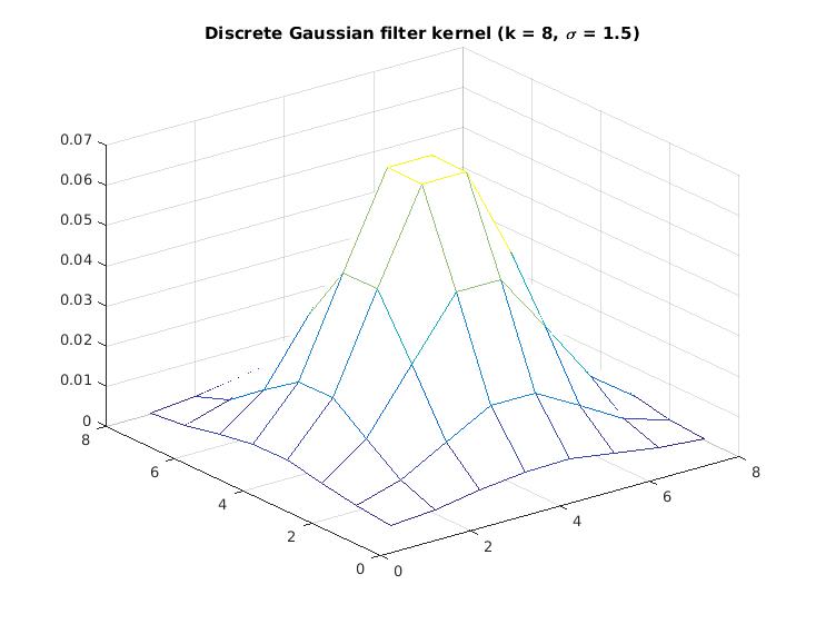
The Gaussian convolution kernel has the effect of smoothing the sharp edges of the heatmap, allowing for a more visually consistent overlay image.

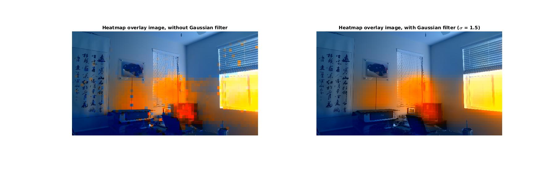
In this approach, the red and blue channels of the entire motion region are offset by a linearly scaled version the standard deviation of the signal of that motion region. A red channel increase/blue channel decrease should correspond to a high standard deviation, whereas a red channel decrease/blue channel increase should correspond to a low standard deviation. In order to "normalize" the standard deviation of all num_horizontal_divisions * num_vertical_divisions signals, the red and blue channel offsets are relative to the average standard deviation across all the signals.

mean_stdev = np.mean(self.heatmap)
...
offset = self.color_intensity_factor * (self.heatmap[vertical_index][horizontal_index] - mean_stdev)
output_image[row][col][2] = self._clip_rgb(output_image[row][col][2] + offset)  # Red channel
output_image[row][col][0] = self._clip_rgb(output_image[row][col][0] - offset)  # Blue channel

Practical applications: Raspberry Pi

I've also included a Python scriptin the repository for Raspberry Pis. It takes a picture on the Pi's camera and saves it to the specified directory with an appropriate file name. I imagine this script can be placed in crontab to take a picture in every specified interval of time while the Pi is stationary, to generate a time-lapse sequence that can be used as input to this algorithm.

Website

Github

Twitter