December 19, 2016 / 2:59 AM
Building An Automated Solver for Facebook Messenger's Brick Pop
projects
Brick Pop
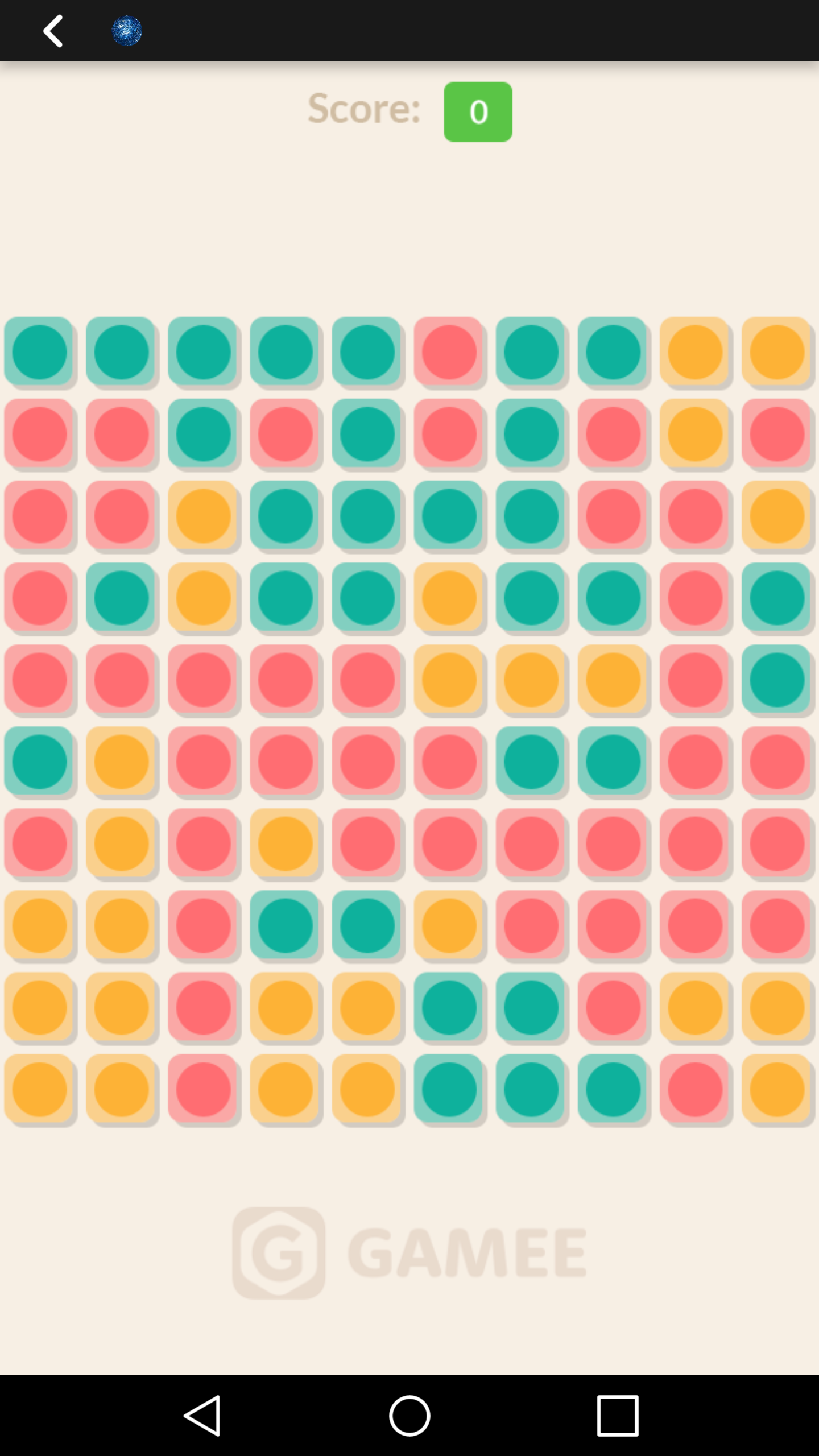
Brick Pop is one of Facebook Messenger's Instant Gameslaunched in the last month. The premise of the game is quite simple: you tap on "bricks" to pop a group of bricks of the same color, until the entire board is cleared. Then, you move on to the next level (with possibly more colors), and this continues presumably indefinitely.
This is all fine and good, but games are more fun when you can automate them and have computers play them for you.
Automation
This project (Github repository) enables total automation of Brick Pop, from generating a solution to the board to playing through the game on a physical, connected Android device.
Defined More Precisely
The game board is a fixed-size, 10x10 square board where each element has either a defined or null color: defined colors correspond to bricks that are still present, and "null" colors correspond to bricks that have been popped. Gameplay itself can be described very precisely by a set of rules governing state transitions; i.e., transitions from one board configuration to another. Effectively, generating a solution reduces down to describing a sequence of state transitions such that the last transition in the sequence causes the board to enter a solved state.
- Popping a brick from any location (i,j)recursively pops all bricks within its flood pool, defined as the set of the origin brick and its neighbors (and their neighbors thereof) who share the same color as the brick at (i,j). The game defines a neighbor of a block at (i,j)to be any block ∈{(i+1,j),(i−1,j),(i,j+1),(i,j−1)}. A pop is considered valid (and thus can only induce a state transition) if the size of the flood pool set is greater than unity.
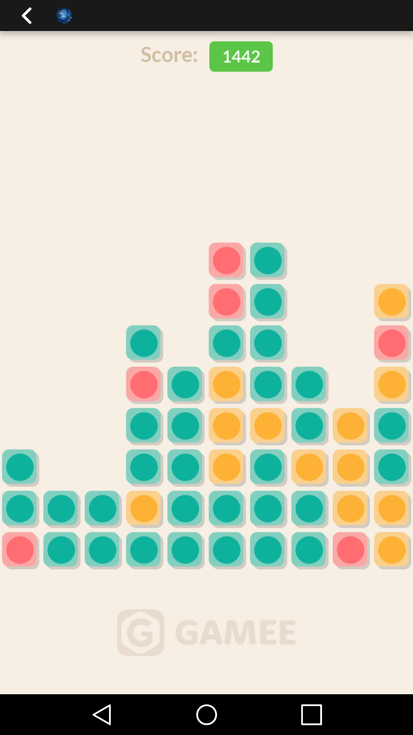
- A contraction process follows each removal of a flood pool. Columns are contracted if every element in the column (after the pop) is null, causing every element in columns to the right to be shifted left into the cleared column. More precisely, a column jconsisting only of empty elements is contracted, causing all elements formerly located at (i,j+1)to have a new location (i,j). Rows are contracted if there exists defined colors anywhere above empty colors; e.g. colored bricks at (i,j)and an empty brick at (i+n,j)for any n>0. The colored bricks are vertically offset to a new index such that no empty elements exist below it.
- The board is considered to be solved state when there are zero non-null elements left on the board. This state can only be reached by a sequence of valid flood pool pops.
With the above state transition rules precisely defined, gameplay itself consists of repeating the flood pop procedure until the board is solved. The challenge here, then, is to define a strategy for generating a valid solution path (i.e. a series of flood pop instructions) that, when executed on the original board, reduces the board to a solved state.
Observations
- The solution search space is very large. Any input board configuration can have up to 10-20 available moves (i.e. valid coordinates at which a flood pool pop can be executed). This number is higher when the board consists of more colors (the maximum such number of unique colors is six) or when the board consists of no null elements (i.e. when the level is first started). The size of the search tree is exponential in size, and any search algorithm that exhaustively explores all possible solutions is necessarily exponential in asymptotic complexity.
- Any input board configuration can have several valid solution paths. Thus, it is wisest to fully explore one potential solution route and check its validity at the end (as in a depth-first search) rather than attempting to fully exhaust exploration of each possible move at each step (as in a breadth-first search). Using DFS allows us to arrive at a solution much faster, but there is no guarantee for a path-length optimized solution (i.e. solving a board in the minimum number of steps).
- The game is structured in such a way that it is difficult to use any heuristics to intelligently traverse the search tree. The gameplay rules are simple; state transitions are pure and can be fully described by any current state of the board. The game does not attempt to be "clever" in any way to suggest that one type of state transition is more likely to solve the board than another. Thus, an automated solution can only optimize the performance of a (worst-case) full traversal of the exponentially-sized search tree.
An Algorithm for Generating a Solution Path
An algorithm to solve the board arises naturally from the insight gained from the above surface-level observations while playing the game as a human. The algorithm must explore the search space using a depth-first traversal, and must reject all solution paths that do not generate a solved board when there are no more available moves for any given board state.
The implementation turns out to be pleasantly simple, requiring only five lines of Python.
def serial_solve(board, steps=tuple([])):
    if board.is_solved():
        return Solution(steps)

    possible_solutions = (
        serial_solve(new_board, steps + (step,))
        for (step, new_board) in board.available_moves()
    )
    valid_solutions = (
        steps
        for steps in possible_solutions
        if not steps.is_empty()
    )

    return next(valid_solutions, EmptySolution())
board.available_moves() returns a list of (step, new_board) describing the coordinate that can be popped and the board configuration that results from that pop. Solution and EmptySolution serve only as containers around values to denote null and non-null values in the same vein as Scala's Some.
For every available move for a board state, the algorithm makes a recursive call to serial_solve to fully exhaust the exploration path of that node. The return value of the function is the first non-null solution path discovered by this traversal, or an EmptySolution is no paths can solve the board. Python generators allow for lazy evaluation of the map, so the implementation doesn't lose out on any performance.
The other non-trivial component of the full implementation is a class that describes the actions of the game board. The Boardclass serves this purpose, with an API including methods pop_from(Coordinate coord), contract(), and is_solved(), to fully simulate the behavior of the actual game. The class is backed by a performant, two-dimensional array whose structure replicates that of the actual game board.
Performance and Parallelism
It becomes quickly apparent that attempting to explore an exponentially-sized solution space is computationally burdensome for any board configuration with more than four colors. However, with observation #2 in mind, a solution can be generated much faster if all available starting points are explored simultaneously. (A serial implementation suffers significantly since an initial starting point may never yield a solution path, yet it must be fully explored before moving on to the next starting point.) Thus, the implementation makes use of process-based parallelism courtesy of Python's multiprocessing module to explore each available move from the initial board configuration in parallel.
def parallel_solve(board):
    queue = multiprocessing.Queue()

    processes = [
        multiprocessing.Process(target=solution_search, args=(queue, [single_start_point],))
        for single_start_point in board.available_moves()
    ]

    for p in processes:
        p.start()

    solution = EmptySolution()
    num_failed_solves = 0
    while True:
        if num_failed_solves >= len(processes):
            break

        try:
            solution = queue.get(block=False)
            if solution.is_empty():
                num_failed_solves += 1
            else:
                break
        except Queue.Empty:
            pass

    for p in processes:
        p.terminate()

    p.join()

    return solution
Since the algorithm is only interested in a single, valid solution, each process has write access to a shared-memory queue initialized in the parent process. When a solution is discovered, this queue is mutated, and the parent accepts this solution and kills all child processes before returning.
In testing, the parallel solver is able to solve most boards in less than 10 seconds, offering a speedup of several orders of magnitude over the serial solver, which would often take hundreds of seconds or may not terminate at all. (Speedup, as a metric of performance, is used loosely in this context: the program is inherently non-deterministic since it does not attempt to fully explore the solution space. Rather, it quits immediately when it encounters the first valid solution, a la the Eureka programming model.)
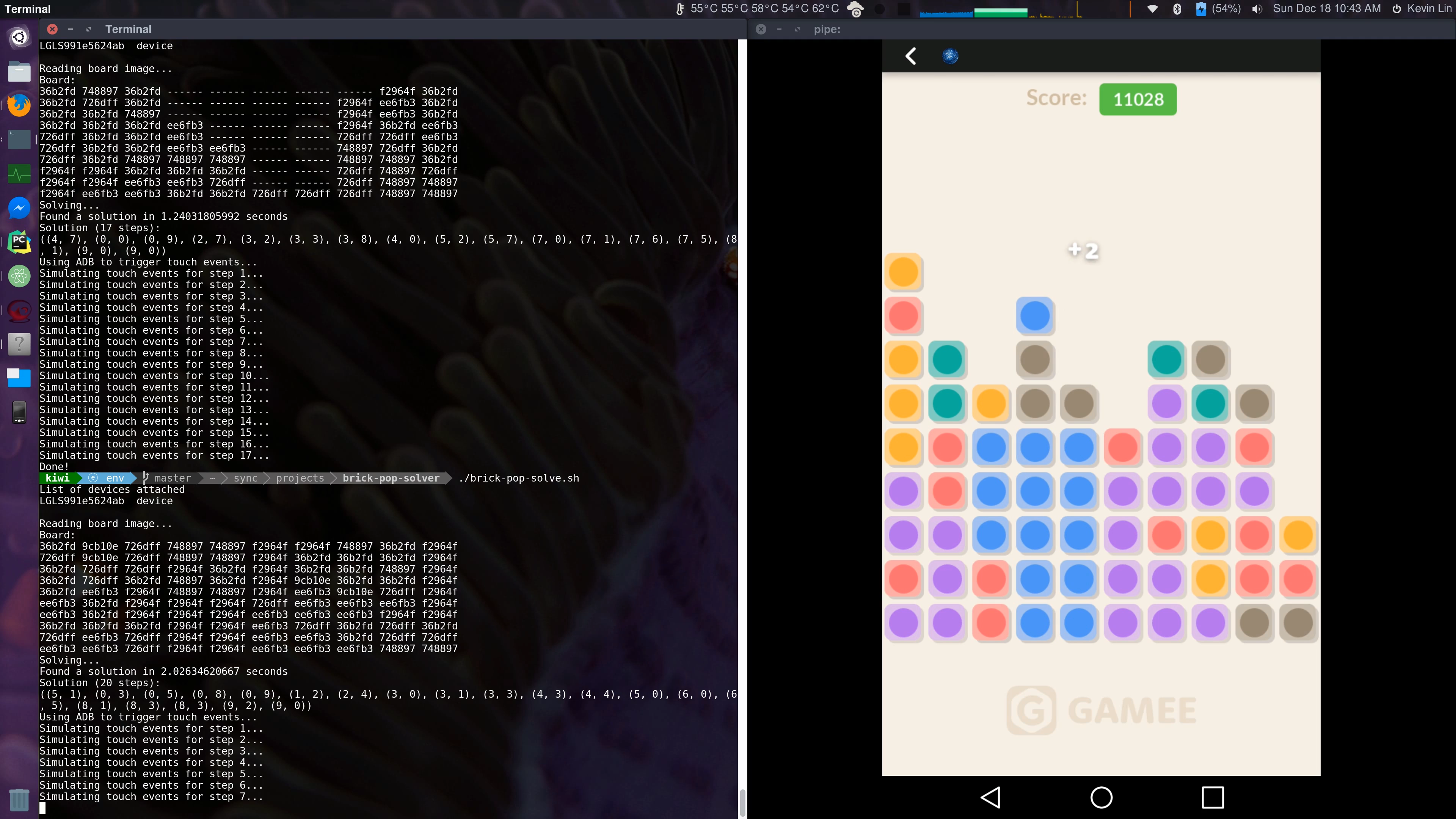
Interface with a Physical Device
With an algorithm in place to generate solution steps and a class to simulate gameplay actions on the board, the last step is automation of gameplay on the physical device. This involves:
- Taking and parsing a screenshot of the board from the device, and creating an appropriate Board instance to describe the input
- Running the solver on the board to generate a sequence of steps to the solution
- Executing the solution on the game board by simulating touch events on the connected device via ADB
Fortunately, Android natively provides an interface to make these tasks painless.
Github
Please see the repository on Githubfor the full source and more information.